Introduction to Model Error Analysis
Principle
After training a ML model, data scientists need to investigate the model failures to build intuition on the critical sub-populations on which the model is performing poorly. This analysis is essential in the iterative process of model design and feature engineering and is usually performed manually.
The mealy package streamlines the analysis of the samples mostly contributing to model errors and provides the user with automatic tools to break down the model errors into meaningful groups, easier to analyze, and to highlight the most frequent type of errors, as well as the problematic features correlated with the failures.
We call the model under investigation the primary model.
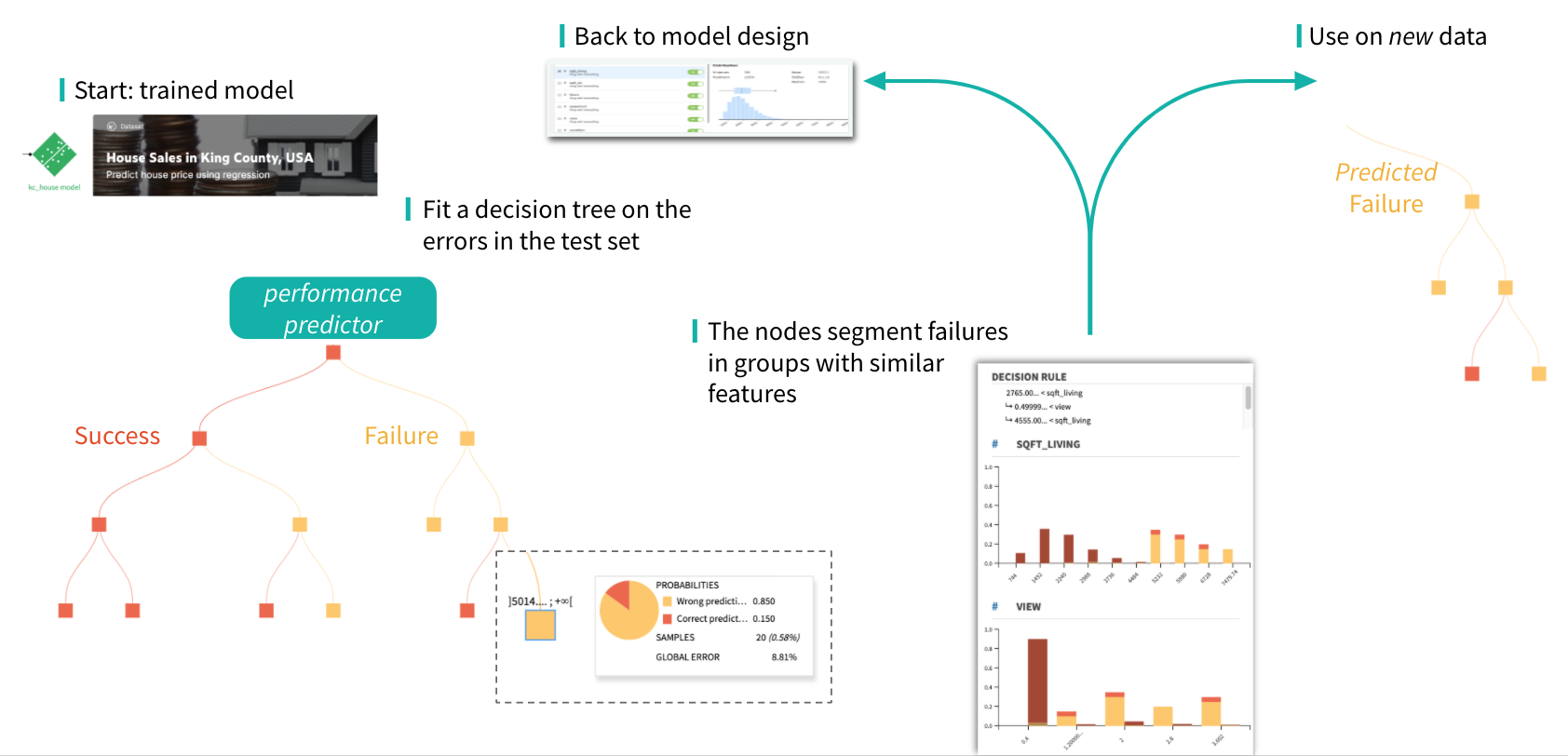
This approach relies on an Error Tree, a secondary model trained to predict whether the primary model prediction is correct or wrong, i.e. a success or a failure. More precisely, the Error Tree is a binary DecisionTree classifier predicting whether the primary model will yield a Correct Prediction or a Wrong Prediction.
The Error Tree can be trained on any dataset meant to evaluate the primary model performances, thus containing ground truth labels. In particular the provided primary test set is split into a secondary training set to train the Error Tree and a secondary test set to compute the Error Tree metrics.
In classification tasks the model failure is a wrong predicted class, whereas in case of regression tasks the failure is defined as a large deviation of the predicted value from the true one. In the latter case, when the absolute difference between the predicted and the true value is higher than a threshold ε, the model outcome is considered as a Wrong Prediction. The threshold ε is computed as the knee point of the Regression Error Characteristic (REC) curve, ensuring the absolute error of primary predictions to be within tolerable limits.
The leaves of the Error Tree decision tree break down the test dataset into smaller segments with similar features and similar model performances. Analyzing the sub-population in the error leaves, and comparing with the global population, provides insights about critical features correlated with the model failures.
The mealy package leads the user to focus on what are the problematic features and what are the typical values of these features for the mis-predicted samples. This information can later be exploited to support the strategy selected by the user :
improve model design: removing a problematic feature, removing samples likely to be mislabeled, ensemble with a model trained on a problematic subpopulation, …
enhance data collection: gather more data regarding the most erroneous under-represented populations,
select critical samples for manual inspection thanks to the Error Tree and avoid primary predictions on them, generating model assertions.
The typical workflow in the iterative model design supported by error analysis is illustrated in the figure below.
Metrics
The actual accuracy of the primary model is the proportion of samples in the test set the primary model predicts correctly (or close enough to the true value in case of regression).
The Error Tree provides an estimation of this accuracy, referred to as estimated accuracy. This is the proportion of samples in the test set the Error Tree estimates as Correct Prediction
If the estimated accuracy of the primary model is too far from the actual one, a warning is triggered. Indeed this means that the decision tree is not representative of the primary model performance, making the whole error analysis invalid. The metric measuring how the Error Tree is representative of the primary model is the Fidelity (1-|actual_acc - estimated_acc|). The chosen threshold for fidelity is 0.9, below which the Error Tree predicted model accuracy is considered too different from the true model accuracy.
As the Error Tree is simply a tree, it can be visualized and further analyzed by looking at its nodes, especially the leaves. The color of a node represents whether the majority of samples falling in the node are Correct Prediction (blue) or Wrong Prediction (red).
In particular the blue leaves represent the subpopulation of the dataset that the primary model managed to predict correctly. Vice versa, the red leaves are the Failure Nodes and represent observations for which the model gives bad predictions. Those points are particularly interesting as they give us insight on the reasons behind the model errors.
There are four informations characterizing a node in the tree:
Correct predictions: number of samples the primary model predicts correctly
Wrong predictions: number of samples the primary model predicts wrongly
Local error: the ratio Wrong / (Wrong + Correct). This is equivalent to the purity of a leaf node of class Wrong prediction.
Fraction of total error: the ratio between the number of errors in this node vs the number of total errors