Active Learning on Digit Recognition with Clustering-based Sampling

We here compare several clustering-based Active Learning approaches and in particular explore the trade-off between speed and performance. For this purpose, we use two standard clustering: a simple KMeans and a MiniBatchKMeans. We compare both of them to Zhdanov’s approach proposed in Diverse mini-batch Active Learning. The author introduced a two-step procedure that first select samples using uncertainty and then performs a KMeans.

Those are the necessary imports and initializations

from matplotlib import pyplot as plt
import numpy as np
from time import time

from sklearn.datasets import load_digits
from sklearn.ensemble import RandomForestClassifier
from sklearn.model_selection import train_test_split
from sklearn.cluster import KMeans

from cardinal.uncertainty import MarginSampler
from cardinal.clustering import KMeansSampler
from cardinal.random import RandomSampler
from cardinal.plotting import plot_confidence_interval
from cardinal.base import BaseQuerySampler
from cardinal.zhdanov2019 import TwoStepKMeansSampler
from cardinal.utils import pad_with_random, ActiveLearningSplitter

np.random.seed(7)

The parameters of this experiment are:

• batch_size is the number of samples that will be annotated and added to the training set at each iteration,

• n_iter is the number of iterations in the simulation.

We use the digits dataset and a RandomForestClassifier.

batch_size = 45
n_iter = 10

X, y = load_digits(return_X_y=True)
X /= 255.
n_samples = X.shape[0]

model = RandomForestClassifier()

A new Custom Sampler

Zhdanov preselects beta * batch_size samples using uncertainty sampling and then uses KMeans to cluster the data in `batch_size clusters and select the samples closest to the cluster centers. By doing this, a diverse set of sample with high uncertainty is selected.

We hypothetize that inversing these steps can also be an interesting approach. For that, we first perform a KMeans clustering, and then select within each cluster the most uncertain samples.

class KMeansClassSampler(BaseQuerySampler):
    def __init__(self, model, n_classes, batch_size):
        self.clustering = KMeans(n_clusters=n_classes)
        self.confidence_sampler = MarginSampler(model, batch_size // n_classes)
        super().__init__(batch_size)

    def fit(self, X_train, y_train):
        self.confidence_sampler.fit(X_train, y_train)
        return self

    def select_samples(self, X):
        self.clustering.fit(X)
        all_samples = set()
        for label in np.unique(self.clustering.labels_):
            indices = np.arange(X.shape[0])
            mask = np.zeros(X.shape[0], dtype=bool)
            mask[self.clustering.labels_ == label] = True
            selected = self.confidence_sampler.select_samples(X[mask])
            all_samples.update(indices[mask][selected])
        return pad_with_random(np.asarray(list(all_samples)), self.batch_size,
                               0, X.shape[0])


class_sampler = KMeansClassSampler(model, 15, 45)

Core Active Learning Experiment

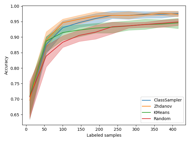
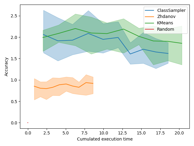
We now compare our class sampler to Zhdanov, a simpler KMeans approach and, of course, random. For each method, we measure the time spent at each iteration and we plot the accuracy depending on the size of the labeled pool but also time spent.

samplers = [
    ('ClassSampler', class_sampler),
    ('Zhdanov', TwoStepKMeansSampler(5, model, batch_size)),
    ('KMeans', KMeansSampler(batch_size)),
    ('Random', RandomSampler(batch_size)),
]

figure_accuracies = plt.figure().number
figure_execution_times = plt.figure().number


for sampler_name, sampler in samplers:

    all_accuracies = []
    all_execution_times = []

    for k in range(10):
        splitter = ActiveLearningSplitter.train_test_split(n_samples, test_size=500, random_state=k)
        splitter.initialize_with_random(batch_size, at_least_one_of_each_class=y[splitter.train], random_state=k)

        accuracies = []
        execution_times = []


        # The classic active learning loop
        for j in range(n_iter):
            model.fit(X[splitter.selected], y[splitter.selected])

            # Record metrics
            accuracies.append(model.score(X[splitter.test], y[splitter.test]))

            t0 = time()
            sampler.fit(X[splitter.selected], y[splitter.selected])
            selected = sampler.select_samples(X[splitter.non_selected])
            splitter.add_batch(selected)
            execution_times.append(time() - t0)

        all_accuracies.append(accuracies)
        all_execution_times.append(execution_times)

    x_data = np.arange(10, batch_size * (n_iter - 1) + 11, batch_size)
    x_time = np.cumsum(np.mean(all_execution_times, axis=0))

    plt.figure(figure_accuracies)
    plot_confidence_interval(x_data, all_accuracies, label=sampler_name)

    plt.figure(figure_execution_times)
    plot_confidence_interval(x_time, all_execution_times, label=sampler_name)


plt.figure(figure_accuracies)
plt.xlabel('Labeled samples')
plt.ylabel('Accuracy')
plt.legend()
plt.tight_layout()

plt.figure(figure_execution_times)
plt.xlabel('Cumulated execution time')
plt.ylabel('Accuracy')
plt.legend()
plt.tight_layout()

plt.show()

• 
• 

Discussion

Accuracies

Let’s start by focusing on the figure showing accuracy depending on the number of labeled samples. We observe that regular KMeans is slightly better at the beginning, probably because it is pure diversity and that exploration is best at the beginning. After that, Zhdanov’s method clearly takes over the other methods.

Execution Times

Execution time is usually not critical in active learning as the query sampling time is negligible compared to labeling time. However, a significant decrease of query sampling time could allow to train more often and thus increase the accuracy of the model faster.

In the plot showing accuracy depending on execution time, we first see a red bar which is the random sampling. This method is almost instantaneous. We also see that the domination of Zhdanov is even more clear. It is because the two-step approach allows to greatly reduce the number of samples on which the KMeans is performed. The difference is small here because we have a small dataset but on a bigger one, the win can be significant. One can also consider using mini-batch KMeans from scikit-learn that is faster.

Estimated memory usage: 22 MB