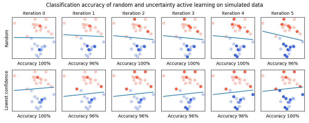
Lowest confidence vs. Random sampling

The simplest way to convince ourselves that active learning actually works is to first test it on simulated data. In this example, we will generate a simple classification task and see how active learning allows to converge faster toward the best result.

Those are the necessary imports and initializations

from matplotlib import pyplot as plt
import numpy as np

from sklearn.datasets import make_blobs
from sklearn.svm import SVC

from cardinal.random import RandomSampler
from cardinal.uncertainty import ConfidenceSampler
from cardinal.utils import ActiveLearningSplitter

np.random.seed(8)

Our simulated data is composed of 2 clusters that are very close to each other but linearly separable. We use as simple SVM classifier as it is a basic classifer.

The parameters of this experiment are:

• n is the number of points in the sumulated data,

• batch_size is the number of samples that will be annotated and added to the training set at each iteration,

• n_iter is the number of iterations in our simulation

n = 30
batch_size = 2
n_iter = 6

X, y = make_blobs(n_samples=n, centers=2,
                  random_state=0, cluster_std=0.80)

model = SVC(kernel='linear', C=1E10, probability=True)

This helper function plots our simulated points in red and blue. The one that are not in the training set are faded. We also plot the linear separation estimated by the SVM.

def plot(a, b, score, selected):
    plt.xlabel('Accuracy {}%'.format(int(score * 100)), fontsize=10)

    # Plot not selected first in low alpha, then selected
    for l, s in [(0, False), (1, False), (0, True), (1, True)]:
        alpha = 1. if s else 0.3
        color = 'tomato' if l == 0 else 'royalblue'
        mask = np.logical_and(selected == s, l == y)
        plt.scatter(X[mask, 0], X[mask, 1], c=color, alpha=alpha)

    # Plot the separation margin of the SVM
    x_bounds = np.array([np.min(X[:, 0]), np.max(X[:, 0])])
    plt.plot(x_bounds, a * x_bounds + b)

Core Active Learning Experiment

As presented in the introduction, this loop represents the active learning experiment. At each iteration, the model learn on all labeled data to measure its performance. The model is then inspected to find out the samples on which its confidence is the lowest. This is done through cardinal samplers.

samplers = [
    ('Random', RandomSampler(batch_size=batch_size, random_state=0)),
    ('Lowest confidence', ConfidenceSampler(model, batch_size))
]

plt.figure(figsize=(10, 4))

for i, (sampler_name, sampler) in enumerate(samplers):
    splitter = ActiveLearningSplitter(X.shape[0])
    splitter.initialize_with_random(2, at_least_one_of_each_class=y)

    for j in range(n_iter):
        model.fit(X[splitter.selected], y[splitter.selected])
        sampler.fit(X[splitter.selected], y[splitter.selected])
        w = model.coef_[0]

        plt.subplot(len(samplers), n_iter, i * n_iter + j + 1)
        plot(-w[0] / w[1], - model.intercept_[0] / w[1], model.score(X, y), splitter.selected.copy())

        selected = sampler.select_samples(X[splitter.non_selected])
        splitter.add_batch(selected)

        if j == 0:
            plt.ylabel(sampler_name)
        plt.axis('tight')
        plt.gca().set_xticks(())
        plt.gca().set_yticks(())
        if i == 0:
            plt.gca().set_title('Iteration {}'.format(j), fontsize=10)

plt.tight_layout()
plt.subplots_adjust(top=0.86)
plt.gcf().suptitle('Classification accuracy of random and uncertainty active learning on simulated data', fontsize=12)
plt.show()

Estimated memory usage: 33 MB