Incremental KMeans

In an active learning setting, the trade-off between exploration and exploitation plays a central role. Exploration, or diversity, is usually enforced using coresets or, more simply, a clustering algorithm. KMeans is therefore used to select samples that are spread across the dataset in each batch. However, to the best of our knowledge, maintaining diversity throughout the whole experiment is something that has not been considered.

By allowing to start the optimization with fixed cluster centers, our Incremental KMeans allows for an optimal exploration of the space since samples are less likely to be selected nearby an already selected sample.

This notebook introduces the principle behind Incremental KMeans and runs a small benchmark on generated data.

from sklearn.cluster import MiniBatchKMeans
from sklearn.metrics import pairwise_distances_argmin_min
from sklearn.ensemble import RandomForestClassifier
from sklearn.model_selection import train_test_split
from cardinal.kmeans import IncrementalMiniBatchKMeans
from cardinal.clustering import MiniBatchKMeansSampler, IncrementalMiniBatchKMeansSampler
from sklearn.datasets import make_blobs
from matplotlib import pyplot as plt
from scipy.stats import ttest_rel
from cardinal.utils import ActiveLearningSplitter
import numpy as np

# Inertia
# ^^^^^^^
#
# Throughout this notebook, we will use the inertia metric, it is the
# euclidean distance from a set of points to a set of center points.


def inertia(data, centers):
    return (pairwise_distances_argmin_min(data, centers)[1] ** 2).sum()



# Active learning like-experiment
# ^^^^^^^^^^^^^^^^^^^^^^^^^^^^^^^
#
# Before digging into the behaviors proper to incremental KMeans, we test
# it in an active learning experiment on simulated data.

X, y, centers = make_blobs(n_samples=10000, centers=100, return_centers=True,
                           n_features=512, random_state=2)

clf = RandomForestClassifier()

kmeans_inertia = []
kmeans_accuracy = []
sampler = MiniBatchKMeansSampler(10)

idx = ActiveLearningSplitter.train_test_split(10000, test_size=.2, random_state=0)
idx.initialize_with_indices(np.arange(10))

for i in range(10):
    selected = sampler.fit(X[idx.selected]).select_samples(X[idx.non_selected])
    idx.add_batch(selected)
    kmeans_inertia.append(inertia(X[idx.test], X[idx.selected]))

    clf.fit(X[idx.selected], y[idx.selected])
    kmeans_accuracy.append(clf.score(X[idx.test], y[idx.test]))


ikmeans_inertia = []
ikmeans_accuracy = []
sampler = IncrementalMiniBatchKMeansSampler(10, random_state=0)

idx = ActiveLearningSplitter.train_test_split(10000, test_size=.2, random_state=0)
idx.initialize_with_indices(np.arange(10))

for i in range(10):

    selected = sampler.fit(X[idx.selected]).select_samples(X[idx.non_selected])

    idx.add_batch(selected)
    ikmeans_inertia.append(inertia(X[idx.test], X[idx.selected]))

    clf.fit(X[idx.selected], y[idx.selected])
    ikmeans_accuracy.append(clf.score(X[idx.test], y[idx.test]))


plt.plot(range(10), kmeans_accuracy, label='KMeans')
plt.plot(range(10), ikmeans_accuracy, label='Incr. KMeans')
plt.ylabel('Accuracy ────')
plt.legend(loc=6)
plt.xlabel('Iteration')

plt.gca().twinx()
plt.gca().set_prop_cycle(None)
plt.plot(range(10), kmeans_inertia, '--')
plt.plot(range(10), ikmeans_inertia, '--')
plt.ylabel('Inertia ╶╶╶╶')

plt.tight_layout(rect=[0, 0.03, 1, 0.95])
plt.show()

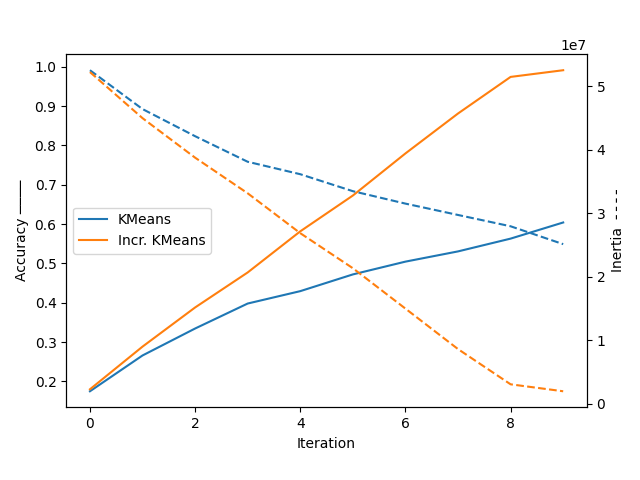
In this simple exemple, we see that Incremental KMeans has a decisive advantage over KMeans because it is able to gradually explore the space of samples.

Analysis of Incremental KMeans

Let us first define the parameters of our experiment. We will generate a dataset from 8 clusters and we will try to keep 4 clusters fixed. We do this example in 2 dimensions for visualization purposes.

n_clusters = 8
n_fixed_clusters = 4

X, y, centers = make_blobs(centers=n_clusters, return_centers=True,
                           n_features=2, random_state=2)

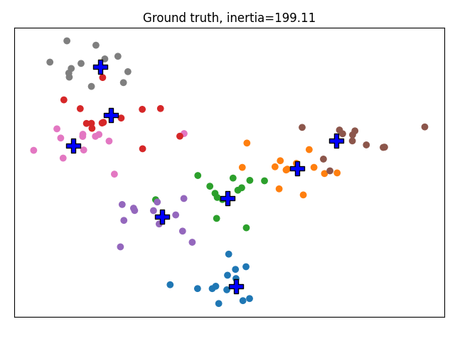
We define plotting functions. This function allows to plot the data colored by clusters, and allows to displays fixed cluster centers in red and regular centers in blue. We use it to display the ground truth.

def plot_clustering(label, y_pred, centers, fixed_centers=[], inertia=None):
    colors = ['C{}'.format(i) for i in y_pred]
    plt.scatter(X[:, 0], X[:, 1], c=colors)
    plt.scatter(centers[:, 0], centers[:, 1], c='blue', edgecolors='k',
                marker='P', s=200)
    if len(fixed_centers) > 0:
        plt.scatter(fixed_centers[:, 0], fixed_centers[:, 1],
                    c='red', edgecolors='k', marker='P', s=200)
    plt.xticks([])
    plt.yticks([])
    plt.tight_layout(rect=[0, 0.03, 1, 0.95])
    if inertia:
        label = label + ", inertia={0:0.2f}".format(inertia)
    plt.title(label)
    plt.show()

plot_clustering('Ground truth', y, centers, inertia=inertia(X, centers))

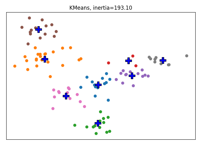
We run a regular MiniBatchKMeans. KMeans would be more suited for this kind of small dataset but we are aiming at using Increment KMeans on large datasets so its implementation relies on MiniBatchKMeans.

kmeans = MiniBatchKMeans(n_clusters=8, random_state=2)
kmeans.fit(X)
plot_clustering('KMeans', kmeans.predict(X), kmeans.cluster_centers_,
                inertia=kmeans.inertia_)

We now consider that we are aware of 4 of the 8 clusters. We fix them in the IncrementalMiniBatchKMeans so that they are strictly enforced.

ikmeans = IncrementalMiniBatchKMeans(n_clusters=8, random_state=2)
ikmeans.fit(X, fixed_cluster_centers=centers[:n_fixed_clusters])
plot_clustering(
    'Incremental KMeans', ikmeans.predict(X),
    centers[n_fixed_clusters:],
    fixed_centers=centers[:n_fixed_clusters],
    inertia=ikmeans.inertia_)

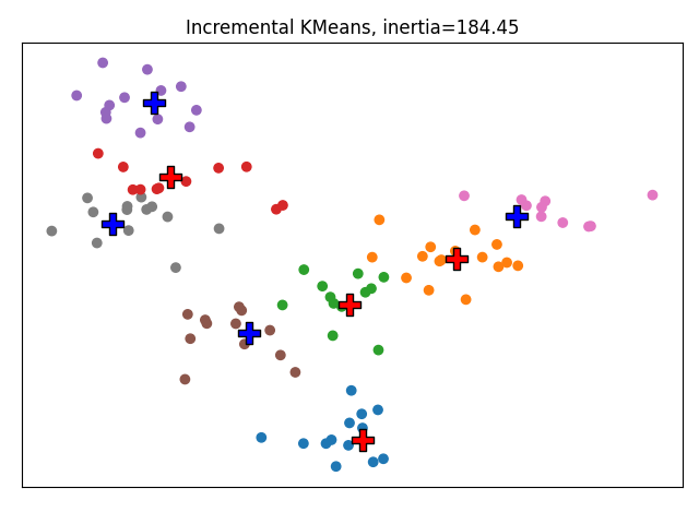
In this basic experiment, we see that the clusters fixed in Incremental KMeans have stayed fixed. We see that the inertia is a little bit lower but this is an effect dependent on the seed. Overall there is no significant difference between the two methods on this toy example.

Experiments in higher dimension

We now want to see the effect of some parameters on the inertia. For this purpose, we repeat the same experiment on a larger dataset with higher dimensions. We explore only a few aspects of the algorithm but our general evaluation function can be used to dig deeper in the algorithm.

The parameter reassignement_ratio is a parameter of the MiniBatchKMeans that controls the ratio of centers of high inertia randomly reassigned

def evaluate(n_samples, n_repeat, n_features, n_blobs, n_clusters,
             n_fixed_clusters, reassignment_ratio):
    inertiae = []
    for i in range(n_repeat):
        X, y, centers = make_blobs(
            centers=n_blobs,
            return_centers=True,
            n_features=n_features,
            random_state=i)
        clus = IncrementalMiniBatchKMeans(
            n_clusters=n_clusters,
            reassignment_ratio=reassignment_ratio
        )
        kwargs = dict()
        kwargs['fixed_cluster_centers'] = None
        if n_fixed_clusters > 0:
            kwargs['fixed_cluster_centers'] = centers[:n_fixed_clusters]
        clus.fit(X, **kwargs)
        inertiae.append(clus.inertia_)
    return inertiae


def plot(xlabel, ylabel, values, inertiae):
    arr = np.asarray(inertiae)
    for i in range(arr.shape[1]):
        plt.scatter(values, arr[:, i], alpha=.4, c='gray')
    plt.plot(values, np.mean(arr, axis=1), c='r')
    plt.xlabel(xlabel)
    plt.ylabel(ylabel)
    plt.show()

Number of fixed cluster centers

In this experiment, we generate data from 10 clusters and see how the number of fixed clusters impacts the inertia.

study_value = []
study_inert = []

for i in range(10):
    study_value.append(i)
    inert = evaluate(5000, 20, 20, 10, 10, i, 0.01)
    study_inert.append(inert)

plot('Number of fixed center clusters /10', 'Mean inertia over 100 runs',
     study_value, study_inert)

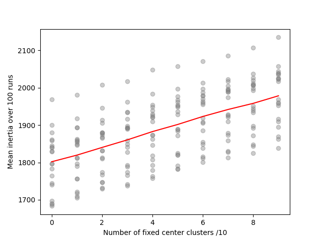
We observe that inertia is proportional to the number of fixed clusters. This happens because fixed clusters are not in a minimum inertia position to start with, so fixing them prevents inertia to be optimized.

Reassignment ratio

We expect the fixed clusters to “get in the way” of clusters trying to move around to reach their cluster. Fortunately, the KMeans++ initialization usually takes care of this by positioning initialization centers in the best areas.

study_value = []
study_inert = []

for i in [0., 0.01, 0.05, 0.1, 0.15, 0.2, 0.3, 0.5]:
    study_value.append(i)
    inert = evaluate(5000, 20, 20, 10, 10, 5, i)
    study_inert.append(inert)

plot('Reassignment ratio', 'Mean inertia over 100 runs',
     study_value, study_inert)

In the end, we observe that the reassignment ratio has absolutely no impact on the intertia which is reassuring.

Estimated memory usage: 115 MB