Measuring hard to classify samples

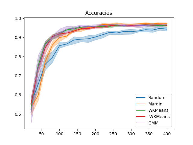
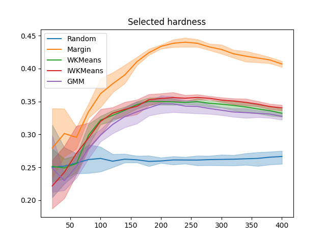
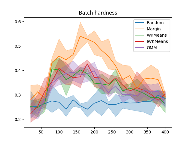
In this example, we run an experiment on real data and try to relate the amount of hard-to-classify samples in the training set with the sampler performance.

from matplotlib import pyplot as plt
import numpy as np

from sklearn.datasets import load_digits
from sklearn.ensemble import RandomForestClassifier
from sklearn.model_selection import RepeatedStratifiedKFold
from sklearn.metrics import pairwise_distances

from cardinal.uncertainty import MarginSampler
from cardinal.clustering import TwoStepIWKMeansSampler, TwoStepGMMSampler
from cardinal.zhdanov2019 import TwoStepKMeansSampler
from cardinal.random import RandomSampler
from cardinal.plotting import plot_confidence_interval
from cardinal.utils import ActiveLearningSplitter

np.random.seed(7)

The parameters of this experiment are:

• batch_size is the number of samples that will be annotated and added to the training set at each iteration,

• n_iter is the number of iterations in our simulation

We use the digits dataset and a RandomForestClassifier as model.

batch_size = 20
n_iter = 20

X, y = load_digits(return_X_y=True)
X /= 255.
n_classes = 10

model = RandomForestClassifier

Core Active Learning Experiment

We now perform the experiment. We compare our adaptive model to random, pure exploration, and pure exploitation. We also monitor the metrics defined above.

samplers = [
    ('Random', lambda clf: RandomSampler(batch_size)),
    ('Margin', lambda clf: MarginSampler(clf, batch_size)),
    ('WKMeans', lambda clf: TwoStepKMeansSampler(10, clf, batch_size)),
    ('IWKMeans', lambda clf: TwoStepIWKMeansSampler(10, clf, batch_size)),
    ('GMM', lambda clf: TwoStepGMMSampler(10, clf, batch_size))
]

all_splitters = dict()
all_accuracies = dict()
all_selected_hardness = dict()
all_batch_hardness = dict()

for i, (sampler_name, sampler_gen) in enumerate(samplers):

    splitters = []
    all_selected_hardness[sampler_name] = []
    all_batch_hardness[sampler_name] = []
    all_accuracies[sampler_name] = []

    for train_idx, test_idx in RepeatedStratifiedKFold(n_splits=2, n_repeats=2, random_state=i).split(X, y):
        splitter = ActiveLearningSplitter(X.shape[0], test_index=test_idx)
        splitter.initialize_with_random(n_classes, at_least_one_of_each_class=y[splitter.train])
        X_test, y_test = X[splitter.test], y[splitter.test]
        clf_trained_on_test = model().fit(X_test, y_test)

        accuracies = []
        batch_hardness = []
        selected_hardness = []

        # The classic active learning loop
        for j in range(n_iter):
            clf = model()
            clf.fit(X[splitter.selected], y[splitter.selected])
            selected_hardness.append(1. - clf_trained_on_test.predict_proba(X[splitter.selected])[np.arange(splitter.selected.sum()), y[splitter.selected]].mean())
            batch_hardness.append(1. - clf_trained_on_test.predict_proba(X[splitter.batch])[np.arange(splitter.batch.sum()), y[splitter.batch]].mean())

            # Record metrics
            accuracies.append(clf.score(X_test, y_test))

            sampler = sampler_gen(clf)
            sampler.fit(X[splitter.selected], y[splitter.selected])
            selected = sampler.select_samples(X[splitter.non_selected])
            splitter.add_batch(selected)

        all_selected_hardness[sampler_name].append(selected_hardness)
        all_batch_hardness[sampler_name].append(batch_hardness)
        all_accuracies[sampler_name].append(accuracies)

# Plot accuracies
plt.figure()
x_data = np.cumsum([batch_size] * n_iter)
for sampler in all_accuracies:
    plot_confidence_interval(x_data, all_accuracies[sampler], label=sampler)
plt.title('Accuracies')
plt.legend()

plt.figure()
x_data = np.cumsum([batch_size] * n_iter)
for sampler in all_selected_hardness:
    plot_confidence_interval(x_data, all_selected_hardness[sampler], label=sampler)
plt.title('Selected hardness')
plt.legend()

plt.figure()
x_data = np.cumsum([batch_size] * n_iter)
for sampler in all_batch_hardness:
    plot_confidence_interval(x_data, all_batch_hardness[sampler], label=sampler)
plt.title('Batch hardness')
plt.legend()

plt.show()

• 
• 
• 

Estimated memory usage: 32 MB