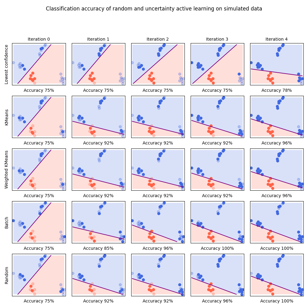
Lowest confidence vs. KMeans sampling

This example shows the importance of diversity-based approaches using a toy example where a very unlucky initialization makes lowest confidence approach underperform.

Those are the necessary imports and initializations

from matplotlib import pyplot as plt
from matplotlib.patches import Polygon
import numpy as np

from sklearn.datasets import make_blobs
from sklearn.svm import SVC

from cardinal.uncertainty import ConfidenceSampler
from cardinal.clustering import KMeansSampler
from cardinal.batch import RankedBatchSampler
from cardinal.random import RandomSampler
from cardinal.utils import ActiveLearningSplitter


np.random.seed(7)

We simulate data where samples of one of the class are scattered in 3 blobs, one of them being far away from the two others. We also select an initialization index where no sample from the far-away sample is initially selected. This will force the decision boundary to stay far from that cluster and thus “trick” the lowest confidence method.

The parameters of this experiment are :

• n is the number of points in the simulated data,

• batch_size is the number of samples that will be annotated and added to the training set at each iteration,

• n_iter is the number of iterations in our simulation.

n = 28
batch_size = 4
n_iter = 5

X, y = make_blobs(n_samples=n, centers=[(1, 0), (0, 1), (2, 2), (4, 0)],
                  random_state=0, cluster_std=0.2)

# We select samples in clusters 0, 1 and 2. Cluster 3 will be ignored by uncertainty sampling
init_idx = [i for j in range(3) for i in np.where(y == j)[0][:2]]
y[y > 1] = 1

model = SVC(kernel='linear', C=1E10, probability=True)

This helper function plots our simulated points in red and blue. The one that are not in the training set are faded. We also plot the linear separation estimated by the SVM.

def plot(a, b, score, selected):

    plt.xlabel('Accuracy {}%'.format(int(score * 100)), fontsize=10)

    l_to_c = {0: 'tomato', 1:'royalblue'}

    f = (lambda x: a * x + b)
    x1, x2 = (np.min(X[:, 0]), np.max(X[:, 0]))
    y1, y2 = (np.min(X[:, 1]), np.max(X[:, 1]))

    # This code computes the coordinates of the background rectangles
    # in order to have pretty prints.
    p1, p2 = (x1, a * x1 + b), ((y1 - b) / a, y1)
    p3, p4 = (x2, a * x2 + b), ((y2 - b) / a, y2)
    p1, p2, p3, p4 = sorted([p1, p2, p3, p4])

    corners = [(x1, y1), (x1, y2), (x2, y2), (x2, y1)]
    dists = [f(x) - y for x, y in corners]
    while dists[0] > 0 or dists[-1] < 0:
        dists.append(dists.pop(0))
        corners.append(corners.pop(0))
    first_pos = next(i for i, x in enumerate(dists) if x > 0)
    plt.gca().add_patch(Polygon(
        [p3, p2] + corners[:first_pos], joinstyle='round',
        facecolor=l_to_c[model.predict([corners[0]])[0]], alpha=0.2))
    plt.gca().add_patch(Polygon(
        [p2, p3] + corners[first_pos:], joinstyle='round',
        facecolor=l_to_c[model.predict([corners[-1]])[0]], alpha=0.2))

    # Plot not selected first in low alpha, then selected
    for l, s in [(0, False), (1, False), (0, True), (1, True)]:
        alpha = 1. if s else 0.3
        mask = np.logical_and(selected == s, l == y)
        plt.scatter(X[mask, 0], X[mask, 1], c=l_to_c[l], alpha=alpha)

    # Plot the separation margin of the SVM
    plt.plot(*zip(p2, p3), c='purple')
    eps = 0.1
    plt.gca().set_xlim(x1 - eps, x2 + eps)
    plt.gca().set_ylim(y1 - eps, y2 + eps)

Core Active Learning Experiment

As presented in the introduction, this loop is the core of the active learning experiment. At each iteration, the model learns on all labeled data to measure its performance. The model is then inspected to find out the samples on which its confidence is the lowest. This is done through cardinal samplers.

In this experiment, we see that lowest confidence will explore the far-away cluster only once all other samples have been labeled. KMeans uses a more exploratory approach and select items in this cluster right away. It is worth noticing that random sampling also have good exploration properties.

samplers = [
    ('Lowest confidence', ConfidenceSampler(model, batch_size)),
    ('KMeans', KMeansSampler(batch_size)),
    ('Weighted KMeans', KMeansSampler(batch_size)),
    ('Batch', RankedBatchSampler(batch_size)),
    ('Random', RandomSampler(batch_size))
]

plt.figure(figsize=(10, 10))

for i, (sampler_name, sampler) in enumerate(samplers):
    splitter = ActiveLearningSplitter(X.shape[0])
    splitter.initialize_with_indices(init_idx)

    for j in range(n_iter):
        model.fit(X[splitter.selected], y[splitter.selected])
        sampler.fit(X[splitter.selected], y[splitter.selected])
        w = model.coef_[0]

        plt.subplot(len(samplers), n_iter, i * n_iter + j + 1)

        if sampler_name == 'Batch':
            weights = ConfidenceSampler(model, batch_size).score_samples(X[splitter.non_selected])
            selected = sampler.select_samples(X[splitter.non_selected], samples_weights=weights)
        elif sampler_name == 'Weighted Kmeans':
            weights = ConfidenceSampler(model, batch_size).score_samples(X[splitter.non_selected])
            selected = sampler.select_samples(X[splitter.non_selected], samples_weights=weights)
        else:
            selected = sampler.select_samples(X[splitter.non_selected])
        splitter.add_batch(selected)

        if j == 0:
            plt.ylabel(sampler_name)
        plt.axis('tight')
        plt.gca().set_xticks(())
        plt.gca().set_yticks(())
        if i == 0:
            plt.gca().set_title('Iteration {}'.format(j), fontsize=10)

        plot(-w[0] / w[1], - model.intercept_[0] / w[1], model.score(X, y), splitter.selected.copy())

plt.tight_layout()
plt.subplots_adjust(top=0.86)
plt.gcf().suptitle('Classification accuracy of random and uncertainty active learning on simulated data', fontsize=12)
plt.show()

Estimated memory usage: 20 MB